Measurement & Uncertainty
No measurement in physics is ever exact — not because experimenters are careless, but because measuring is fundamentally a physical process with limits built into it. This lesson names those limits precisely, since the vocabulary here trips up more students than the actual ideas do.
Every measurement carries some uncertainty
Measure the length of your desk with a ruler ten times, being as careful as you like, and you will not get exactly the same number all ten times. Maybe you'll get 84.6 cm nine times and 84.7 cm once. That tiny spread isn't a sign you're bad at using a ruler — every instrument has a limit to how finely it can distinguish one value from a neighbouring one, and every human reading that instrument adds a little variability of their own. Physics builds a careful vocabulary for describing exactly how much doubt surrounds a given number, and that vocabulary is what this lesson is about.
Two families of error: random and systematic
Errors in measurement split into two categories that behave completely differently, and mixing them up is one of the most common mistakes in this topic.
Random errors cause repeat readings to scatter unpredictably above and below the true value. Causes include your reaction time varying slightly each time you start a stopwatch, tiny fluctuations in how you line your eye up with a scale, or genuine small fluctuations in the thing you're measuring. Because random errors push a reading up just as often as down, their effect shrinks the more times you repeat the measurement and average — a scatter of readings averages out to something much closer to the true value than any single reading would give. This is precisely why repeating an experiment and taking a mean is worth doing: a direct, practical defence against random error.
Systematic errors, by contrast, shift every reading in the same direction by roughly the same amount. A top-pan balance that hasn't been zeroed properly adds the same few grams to every mass measured on it. A stopwatch with a consistent late-start habit makes every timed interval read slightly high. However carefully you repeat a measurement affected by a systematic error, averaging does nothing to fix it — all readings are wrong in the same way, so their average is too. Catching a systematic error usually means comparing your method or instrument against something independent: calibrating the balance against a known mass, timing against a second independent clock, or trying a different experimental method and seeing whether the two agree.
Random error scatters your readings around the true value — fix it by repeating and averaging. Systematic error drags every reading off in the same direction — fix it by recalibrating the instrument or checking against an independent method. Repeating the measurement will never reveal a systematic error, because it repeats the mistake along with the reading.
Precision, accuracy, repeatability, reproducibility, resolution
These five words get used loosely in everyday speech, which is why physics insists on pinning each one down separately. Confusing these terms is one of the most common ways marks get lost in this topic.
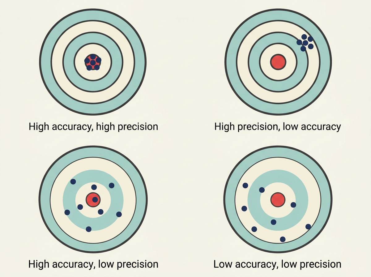
Accuracy describes how close a measurement (or the mean of several measurements) is to the true value. A measurement can be wildly imprecise — a huge scatter of readings — and still be accurate on average, if that scatter is centred on the true value.
Precision describes how close a set of repeated measurements are to each other, regardless of whether they're anywhere near the true value. A tight cluster of readings is precise even if it sits nowhere near the correct answer — that's what a systematic error does: it takes a precise set of readings and shifts the whole cluster off target.
Repeatability refers to how well you can reproduce a result by repeating the measurement yourself, with the same method, equipment and conditions, shortly afterwards. It's a check on your own procedure: five readings in a row under identical conditions coming out very similar means your method is repeatable.
Reproducibility is the same idea stretched further — whether a result can be obtained again when repeated by someone else, using different equipment, in a different lab, possibly with a different method entirely. Reproducibility gives a result real scientific weight, since it shows the result doesn't depend on some quirk of one particular setup or experimenter.
Resolution is a property of the measuring instrument itself: the smallest change in a quantity it can actually detect and display. A ruler marked in millimetres has a resolution of 1 mm; a digital thermometer that only displays whole degrees has a resolution of 1 °C no matter how stable the temperature actually is. Resolution puts a hard floor under how small your uncertainty can possibly be — you cannot claim a smaller uncertainty than your instrument can resolve.
You need a working rule for turning "resolution" into an actual $\pm$ figure, and two situations cover almost everything you'll meet in this course:
Single reading: if you only take one reading, the absolute uncertainty is $\pm$half the smallest scale division — half the resolution. A ruler marked in millimetres gives a single length reading an uncertainty of $\pm0.5\,\text{mm}$, the most the true value could plausibly differ before you'd have noticed it looked different.
Repeated readings: if you take several readings and they don't all agree, use half the range instead: $\text{uncertainty} = \dfrac{\text{max} - \text{min}}{2}$. This captures the actual spread observed, often bigger than the instrument's resolution alone once random error and human variability are included.
Quantifying uncertainty: absolute, fractional, percentage
Once you've accepted that every measurement has some uncertainty attached, the next step is putting a number on it. There are three related ways of expressing that number, and you should be comfortable converting between all three.
The absolute uncertainty is the uncertainty expressed in the same units as the measurement itself. If you measure a length as $12.4\,\text{cm}$ and judge the uncertainty to be $\pm0.1\,\text{cm}$, then $0.1\,\text{cm}$ is the absolute uncertainty, usually written directly after the measurement: $l = (12.4 \pm 0.1)\,\text{cm}$.
The fractional uncertainty strips the units away by dividing the absolute uncertainty by the measured value itself:
For the length above, that's $0.1/12.4 \approx 0.008$. Fractional uncertainty is dimensionless — a pure ratio — which is why it's the form used when combining uncertainties from different quantities with different units, covered in the next lesson.
The percentage uncertainty is the fractional uncertainty multiplied by 100:
For that same length, $0.008 \times 100\% \approx 0.8\%$. Percentage uncertainty tends to be the most intuitive of the three, since it gives an immediate feel for how significant the uncertainty is relative to the measurement, without needing to know the units involved.
The same absolute uncertainty means very different things depending on the size of the measurement. An uncertainty of $\pm1\,\text{mm}$ on a length of $10\,\text{mm}$ is a huge $10\%$ — but the same $\pm1\,\text{mm}$ on a length of $2\,\text{m}$ is a negligible $0.05\%$. This is why percentage and fractional uncertainty matter: they let you judge how serious an uncertainty actually is, rather than being misled by the raw absolute number.
Significant figures as a silent uncertainty statement
The number of significant figures quoted for a value is itself an implicit claim about how well you know it, even without writing "$\pm$" anywhere. Writing a measured length as $12\,\text{cm}$ suggests an uncertainty of around $\pm1\,\text{cm}$; writing it as $12.4\,\text{cm}$ suggests $\pm0.1\,\text{cm}$; writing $12.40\,\text{cm}$ suggests $\pm0.01\,\text{cm}$. Adding digits you don't actually know — writing $12.437291\,\text{cm}$ when your ruler can only resolve millimetres — doesn't make a measurement more accurate. It misrepresents how well you actually know the value, arguably worse than being vague, since it looks precise without being precise.
A useful habit is to match the significant figures in your final answer to the precision actually justified by your least well-known input value, and to quote an explicit $\pm$ uncertainty whenever you can, rather than leaving the reader to infer it from digit count.
When a calculated quantity combines several measurements of different precision, quote the final answer to the same number of significant figures as the least precise measurement that went into it — not the most precise one. Carrying extra digits from a more precise input doesn't rescue the precision lost from a less precise one.
Key takeaways
- Random errors scatter repeat readings unpredictably around the true value and are reduced by repeating the measurement and averaging.
- Systematic errors shift every reading in the same direction by a similar amount and are only caught by recalibrating equipment or comparing against an independent method — repetition alone never fixes them.
- Accuracy is closeness to the true value; precision is closeness of repeated readings to each other — a result can be precise without being accurate.
- Repeatability is consistency under the same method and conditions; reproducibility is consistency when the measurement is repeated independently, by someone else or with different equipment.
- Resolution is the smallest change an instrument can actually detect, and it puts a hard lower limit on how small your quoted uncertainty can be.
- Estimate absolute uncertainty as ±half the smallest scale division for a single reading, or ±half the range (max − min)/2 for repeated readings.
- Absolute uncertainty carries units; fractional uncertainty is absolute uncertainty divided by the measured value; percentage uncertainty is the fractional uncertainty × 100%.
- The number of significant figures quoted for a value is itself an implicit statement about its uncertainty — don't write down digits you don't actually know.
- A calculated quantity should be quoted to the same number of significant figures as the least precise measurement used to find it — extra digits from a more precise input don't buy back lost precision elsewhere.