Combining Uncertainties
A single measured quantity carries its own uncertainty, but almost nothing in physics is used on its own — you multiply lengths together, divide voltages by currents, square velocities. So once you combine several uncertain quantities into a calculation, what happens to their uncertainties? The rules are refreshingly simple, and worth understanding rather than just memorising.
Three rules for propagating uncertainty
Suppose you've measured two quantities, each with its own uncertainty, and need to combine them into a calculated result. There are three situations you'll meet constantly, each with its own rule for how the uncertainty carries through.
When you add or subtract two measured quantities, their absolute uncertainties add — regardless of whether you're adding or subtracting the quantities themselves. If $x = (5.0\pm0.2)\,\text{cm}$ and $y=(3.0\pm0.1)\,\text{cm}$, then whether finding $x+y$ or $x-y$, the uncertainty in the result is $0.2+0.1=0.3\,\text{cm}$. This might feel odd for subtraction, but uncertainty represents the worst case in either direction, and subtracting doesn't make you more certain about either original measurement.
When you multiply or divide two measured quantities, their percentage (or fractional) uncertainties add. If a current $I$ has a percentage uncertainty of $2\%$ and a resistance $R$ has $3\%$, then $V=IR$ carries a percentage uncertainty of $2\%+3\%=5\%$. The derivation below shows exactly where this comes from.
When a measured quantity is raised to a power $n$, its percentage uncertainty is multiplied by $n$. If a radius $r$ has a percentage uncertainty of $1\%$, a volume proportional to $r^3$ has $3\times1\%=3\%$, since $r^3$ is really $r\times r\times r$, and the multiplication rule applies three times over.
Fractional uncertainties add because uncertainty in a product comes from both factors being uncertain at once, and to first order those two contributions just stack. This also explains the power rule — raising to the power $n$ is multiplying a quantity by itself $n$ times, so its fractional uncertainty gets added to itself $n$ times, the same as multiplying by $n$.
Showing uncertainty on a graph: error bars
Once you've got uncertain values for several data points, plotting them needs a way of showing that uncertainty visually rather than just as a single dot. This is what an error bar does — a short line through each plotted point, extending above and below (uncertainty in $y$) or left and right (uncertainty in $x$), its length representing the range within which the true value could plausibly lie. A large uncertainty gets a long error bar; a confidently measured point gets a short one, or none if the uncertainty is too small to show at the graph's scale.
The sizing rule is entirely literal: the bar runs from (value − uncertainty) to (value + uncertainty). A reading of $(5.0\pm0.2)\,\text{cm}$ gets an error bar from $4.8\,\text{cm}$ to $5.2\,\text{cm}$, centred on the plotted point — no scaling needed, just the endpoints given directly by the measurement and its stated uncertainty.
Error bars turn a graph from a simple connect-the-dots exercise into something that honestly represents the quality of your data — and, as the next section shows, they're the basis for working out the uncertainty in a line's gradient and intercept.
Uncertainty in a gradient and intercept
When you fit a straight line through data points, the standard approach is to draw the line of best fit — the single straight line passing as close as possible to every point overall. But that best-fit line alone tells you nothing about how uncertain its gradient or intercept are. For that, you need the error bars.
The method is to draw two further lines, both still consistent with the data: the steepest straight line that can still pass through every error bar, and the shallowest line that can likewise still pass through every error bar. Both are lines the data cannot rule out — the extremes of what's plausible given the scatter and size of your error bars, with the best-fit line sitting somewhere between them.
Find the gradient of each of these two extreme lines; the uncertainty in the gradient is half the difference between them:
The same idea applies to the $y$-intercept: read off the intercept of each extreme line and take half the difference as the uncertainty in the intercept. Half the spread between the two extreme, still-plausible lines is a sensible measure of how much the true gradient (or intercept) could reasonably differ from the one read off the best-fit line alone.
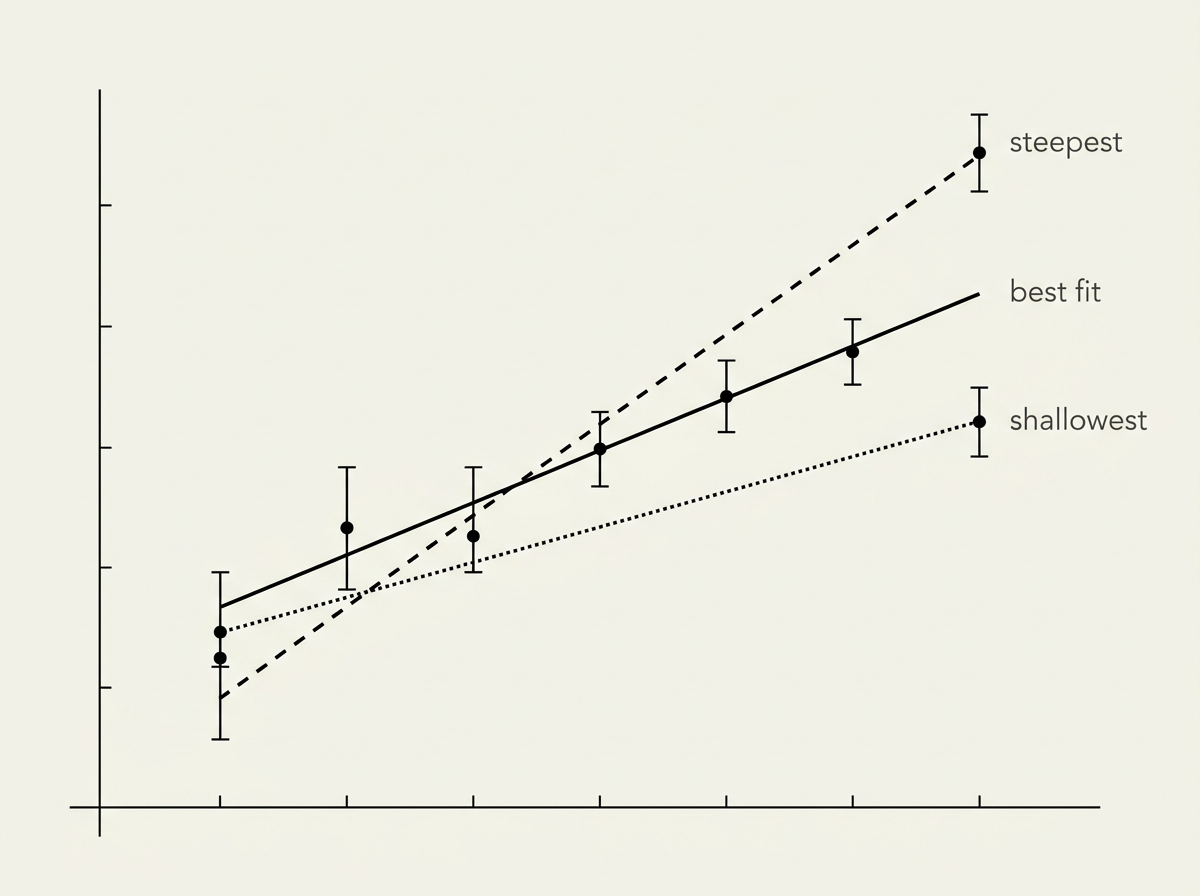
The steepest and shallowest lines must still pass through every error bar, not just through the first and last data points. It's tempting to just pick the two most extreme-looking points and draw between them, but a genuinely valid steepest or shallowest line has to remain consistent with the full set of error bars across the whole graph.
Key takeaways
- When adding or subtracting measured quantities, their absolute uncertainties add, even when the quantities themselves are being subtracted.
- When multiplying or dividing measured quantities, their percentage (or fractional) uncertainties add.
- When a quantity is raised to a power $n$, its percentage uncertainty is multiplied by $n$.
- The multiplication rule can be derived directly from expanding $(x+\Delta x)(y+\Delta y)$ and discarding the negligible second-order term $\Delta x\Delta y$.
- Error bars on a graph show the plausible range of a plotted value, horizontally and/or vertically.
- The uncertainty in a best-fit line's gradient is half the difference between the gradients of the steepest and shallowest lines that still pass through every error bar; the same method gives the uncertainty in the intercept.
- An error bar for a reading of $(5.0\pm0.2)\,\text{cm}$ runs literally from $4.8\,\text{cm}$ to $5.2\,\text{cm}$ — the endpoints are just the value minus and plus its stated uncertainty.