Physics · Mechanics · AS Level

Motion Graphs & Equations of Motion

Watch a ball bounce and you're watching a live demonstration of everything in this lesson — a changing height, a changing speed, and a constant downward acceleration all playing out in front of you. Once you can read that motion off a graph, and calculate it with a handful of equations, you have the working vocabulary for the rest of mechanics.

10 min read

Displacement, velocity and acceleration

Distance is the total length of the path travelled — a scalar, always positive. Displacement is the straight-line distance from the starting point to the current position, plus a direction — a vector, which can be zero even after travelling a large distance, if you return to your start.

Speed is how fast distance is being covered — a scalar. Velocity is the rate of change of displacement — a vector, defined as:

$v = \dfrac{\Delta s}{\Delta t}$

where $\Delta s$ is the change in displacement and $\Delta t$ is the time taken. Acceleration is the rate of change of velocity:

$a = \dfrac{\Delta v}{\Delta t}$

As written, both give average values over $\Delta t$. The instantaneous value at a specific moment is what you get as $\Delta t$ shrinks toward zero — graphically, the difference between the slope of a chord and the slope of a tangent, which is exactly where motion graphs come in.

Reading displacement-time graphs

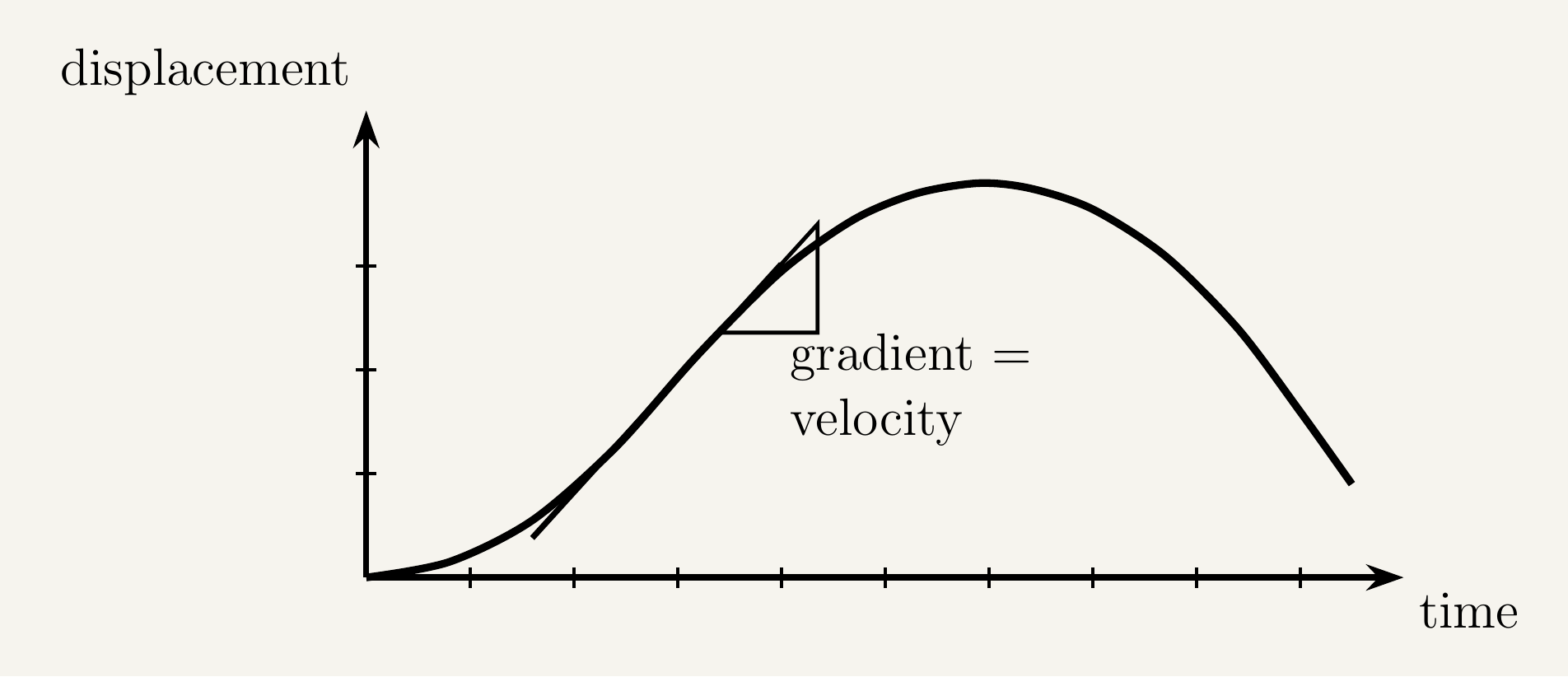
On a displacement-time graph, the gradient at any point is the velocity at that instant, directly from $v = \Delta s/\Delta t$.

A straight-line section means constant velocity. A curved section means the object is accelerating: steepening means speeding up, flattening means slowing down, and a horizontal section (zero gradient) means stationary. A bouncing ball's displacement-time graph curves steeply as it falls and speeds up, flattens briefly at the peak of each bounce, then curves again as it falls once more.

A displacement-time graph titled at the top, with the vertical axis labelled displacement and the horizontal axis labelled time. A single smooth curve rises from the origin, climbs to a rounded peak, then descends. Two short straight tangent lines touch the curve at two different points: one on the rising section, where a small right-angled gradient triangle beside the tangent is labelled gradient = velocity; and one on the falling section past the peak, where a second gradient triangle is labelled gradient = velocity (negative here), showing that a downward-sloping tangent corresponds to a negative velocity. — The gradient of a displacement-time graph at any instant gives the velocity at that instant — positive where the curve rises, negative where it falls.

Reading velocity-time graphs

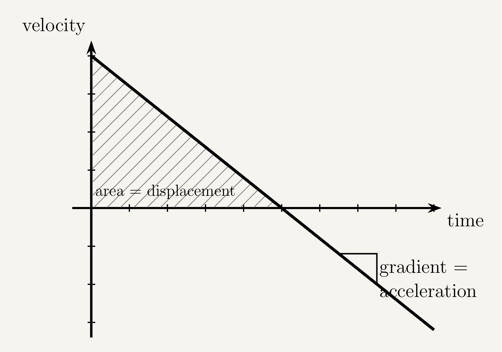
A velocity-time graph carries two pieces of information. The gradient gives the acceleration, from $a = \Delta v/\Delta t$: steeper means a bigger acceleration, horizontal means constant velocity, and a straight sloped line means constant, uniform acceleration.

Second, the area under a velocity-time graph, between two times, equals the displacement over that interval. This follows because area under a constant-velocity line is (velocity) × (time) — exactly displacement for constant velocity — and extends to curved sections by treating the area as many thin rectangles. A bouncing ball's velocity-time graph is a sawtooth: steadily increasing speed during each fall, then jumping to a smaller upward speed at each bounce.

A velocity-time graph titled at the top, with the vertical axis labelled velocity (with an upward arrowhead) and the horizontal axis labelled time (with a rightward arrowhead). A single straight diagonal line starts high on the velocity axis and slopes steadily downward, crossing the time axis partway across and continuing into negative velocity values. The triangular region between the line, the vertical axis and the horizontal axis, from the start up to where the line crosses the time axis, is shaded with diagonal hatching and labelled area = displacement. Further along the line, past where it crosses the time axis, a small right-angled gradient triangle sits beside the line, labelled gradient = acceleration. — The area under a velocity-time graph gives the displacement over that interval; the gradient of the same graph gives the acceleration.

Reading acceleration-time graphs

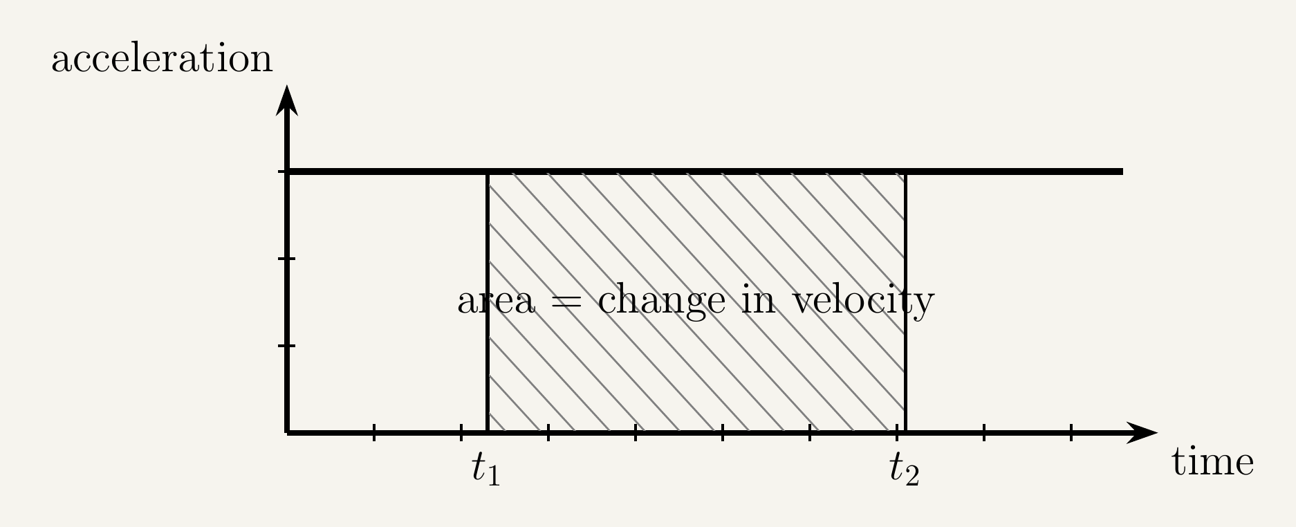
The same logic applies one level up: the area under an acceleration-time graph gives the change in velocity over that interval. For a bouncing ball, ignoring the instant of contact with the floor, the acceleration-time graph is a flat horizontal line at $-g$ throughout each flight, since gravity acts the same whether the ball is moving up or down.

An acceleration-time graph titled at the top, with the vertical axis labelled acceleration and the horizontal axis labelled time, both with small arrowheads. A single straight horizontal line sits at a constant height above the time axis, representing uniform acceleration. The rectangular region between the line, the time axis, and two vertical boundary lines marking a start and end time is shaded with light diagonal hatching and labelled area = change in velocity. — The area under an acceleration-time graph gives the change in velocity over that interval — the same logic as area under a velocity-time graph giving displacement.

Deriving the equations of motion

For uniform (constant) acceleration — including anything falling freely under gravity — the relationships between displacement, velocity, acceleration and time compress into four standard equations, the SUVAT equations after their letters: $s$ (displacement), $u$ (initial velocity), $v$ (final velocity), $a$ (acceleration), $t$ (time). They all follow directly from one another:

DerivationThe four equations of motion for uniform acceleration

Start from the definition of acceleration as the rate of change of velocity: $a = \dfrac{v-u}{t}$, where $u$ is the velocity at the start of the interval and $v$ is the velocity at the end, after time $t$.

This uses the definition directly — for constant acceleration, the average rate of change over the whole interval equals the (constant) acceleration itself.

Rearranging for $v$ gives the first equation of motion: $v = u + at$.

Now consider the velocity-time graph for this motion: a straight line rising from $u$ to $v$ over time $t$ (straight, because acceleration is constant). The displacement is the area under this line, which is the area of a trapezium with parallel sides $u$ and $v$ and width $t$.

This is exactly the "area under a velocity-time graph gives displacement" rule from earlier in this lesson, applied to the specific case of a straight-line graph.

A velocity-time graph showing a single straight line rising from a starting height u on the vertical velocity axis to a higher final height v, over a width t along the horizontal time axis. Dashed guide lines mark the starting height u and the final height v on the velocity axis, and a double-headed arrow beneath the time axis marks the width t. The region between the line, the vertical axis, the horizontal axis and the vertical line at time t is shaded with diagonal hatching and labelled area = s, showing that the displacement is the area of this trapezium. — The velocity-time graph for uniform acceleration: a straight line from u to v over time t, whose area — a trapezium with parallel sides u and v and width t — gives the displacement s.

The area of a trapezium is the average of the two parallel sides multiplied by the width, giving the second equation of motion: $s = \dfrac{(u+v)}{2}t$.

To eliminate $v$ from this equation, substitute $v = u+at$ (from step 2) into $s = \frac{1}{2}(u+v)t$: $s = \frac{1}{2}\big(u + (u+at)\big)t = \frac{1}{2}(2u+at)t$.

Expanding gives the third equation of motion: $s = ut + \dfrac{1}{2}at^2$.

This version is useful whenever you know $u$, $a$ and $t$ but not $v$.

Finally, to find a relationship that doesn't involve time at all, take $v=u+at$ and $s=\frac{1}{2}(u+v)t$ together and eliminate $t$ between them. From the first, $t = \dfrac{v-u}{a}$; substitute this into the second: $s = \dfrac{1}{2}(u+v)\cdot\dfrac{v-u}{a}$.

$(u+v)(v-u)$ is a difference of two squares, which is what makes this substitution simplify so cleanly.

Expanding the numerator: $(u+v)(v-u) = v^2-u^2$, so $s = \dfrac{v^2-u^2}{2a}$, which rearranges to the fourth equation of motion: $v^2 = u^2 + 2as$.

This one is invaluable whenever time isn't given (or isn't asked for) in a problem.

$\begin{array}{r l} \text{1.} & v = u+at \\[6pt] \text{2.} & s = \tfrac12(u+v)t \\[6pt] \text{3.} & s = ut+\tfrac12at^2 \\[6pt] \text{4.} & v^2 = u^2+2as \end{array}$

▪ derived

Worked exampleChoosing the right SUVAT equation

A car accelerates uniformly from $8\,\text{m}\,\text{s}^{-1}$ to $20\,\text{m}\,\text{s}^{-1}$ over a distance of $98$ m. Find its acceleration.

List what's given: $u=8$, $v=20$, $s=98$, and $a$ is wanted — $t$ is neither given nor asked for.

With $u$, $v$, $s$ known and $t$ absent, the equation that fits is $v^2 = u^2+2as$.

Choosing the equation is just matching which four of the five SUVAT letters appear in the question.

Substituting: $20^2 = 8^2 + 2a(98)$, so $400 = 64 + 196a$.

$196a = 336$, giving $a = \dfrac{336}{196} = 1.71\,\text{m}\,\text{s}^{-2}$ (to 3 s.f.).

▪ answer

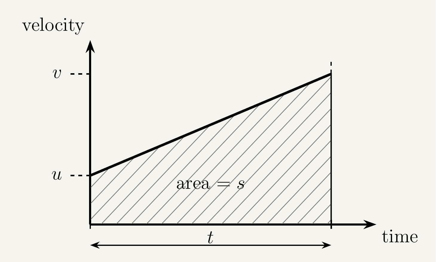
All four equations require the acceleration to be constant over the interval — real motion like a bouncing ball is only uniformly accelerated between bounces, not across the whole trajectory. One value of $a$ recurs constantly: $g$, the acceleration due to gravity near the Earth's surface, roughly $9.81\,\text{m}\,\text{s}^{-2}$ downward for any object in free fall. Unlike the gravitational constant $G$, $g$ isn't truly universal — it varies from about $9.78\,\text{m}\,\text{s}^{-2}$ at the equator to $9.83\,\text{m}\,\text{s}^{-2}$ at the poles, and drops slightly with altitude; $9.81\,\text{m}\,\text{s}^{-2}$ is the standard UK-latitude value.

Sign convention

Pick one direction as positive before starting a SUVAT problem — often "upward" or "the direction of initial motion" — and apply it consistently, including to acceleration, which is often negative. A fifth variant, $s = vt - \frac{1}{2}at^2$, eliminates $u$ instead of $v$ and is handy when $v$ is given rather than $u$.

Required Practical: Determination of g by a Free-Fall Method

AQA Required Practical

This is AQA's Required Practical 3: determining $g$ by timing free fall.

Equipment

Equipment	Purpose
Electromagnet	Holds the ball bearing in place, then releases it cleanly on demand
Steel ball bearing	Dense, small, falls with negligible air resistance over the distances used
Trapdoor switch	Stops the timer automatically the instant the ball lands on it
Electronic (millisecond) timer	Times the fall precisely, without relying on human reaction time
Retort stand and clamp	Holds the electromagnet at a fixed, adjustable height
Metre ruler / tape measure	Measures the fall height $h$, fixed vertically alongside the drop
Switch box	Simultaneously cuts the electromagnet's current and starts the timer

Method

MethodFinding g from h against t²

Clamp the electromagnet at a measured height above a trapdoor switch connected to the electronic timer, and attach the steel ball bearing to the electromagnet.

Measure the fall height $h$ — from the bottom of the ball to the trapdoor — with a vertically fixed metre ruler, reading at eye level to avoid parallax error.

Operate the switch box to simultaneously cut the electromagnet's current (releasing the ball) and start the timer.

The ball falls freely and strikes the trapdoor, which stops the timer automatically — record the fall time $t$.

Repeat the drop at the same height three times and average $t$, to reduce random timing error.

Repeat steps 2–5 for a range of different heights $h$ (five or six values spanning as wide a range as the apparatus allows).

Since $s=ut+\frac12at^2$ with $u=0$ gives $h=\frac12gt^2$, plot $h$ against $t^2$ — a straight line through the origin with gradient $g/2$, so $g$ is found from twice the gradient.

▪ method

Sources of error and how to minimise them

A "sticky" release from residual magnetism

Leftover magnetism can hold the ball back for a fraction of a second after the current is cut, biasing every timing low. Check for a clean, immediate release, and briefly reverse the current between drops to demagnetise the core.

Inconsistent reference point for measuring h

Measuring to a different point on the ball each time introduces a constant offset error. Always measure to the same point — typically the bottom, matching where it triggers the trapdoor.

Air resistance

Normally negligible: a dense, small steel ball falling a short lab distance never gets close to terminal velocity, so drag stays much smaller than weight throughout.

Timing error eliminated by design

A hand-operated stopwatch would introduce a reaction-time error of the same order as the fall time itself. The electromagnet-and-trapdoor circuit removes this by starting and stopping the timer automatically.

Key takeaways

Distance and speed are scalars; displacement and velocity are the corresponding vectors, needing a direction as well as a size.
Velocity is defined as $v = \Delta s/\Delta t$ and acceleration as $a = \Delta v/\Delta t$ — both give average values over the interval unless that interval is shrunk to an instant.
On a displacement-time graph, gradient = velocity; straight sections mean constant velocity, curved sections mean changing velocity (acceleration).
On a velocity-time graph, gradient = acceleration, and the area under the graph = displacement.
On an acceleration-time graph, the area under the graph = change in velocity.
The four SUVAT equations — $v=u+at$, $s=\frac{1}{2}(u+v)t$, $s=ut+\frac12at^2$, $v^2=u^2+2as$ — all follow from the definition of acceleration and the trapezium area under a velocity-time graph, and only apply when acceleration is constant.
$g$, the acceleration due to gravity, is simply a specific, very common value of $a$ that will reappear throughout the rest of the course — but unlike the gravitational constant $G$, $g$ isn't truly universal, varying slightly (roughly $9.78$–$9.83\,\text{m}\,\text{s}^{-2}$) with latitude and altitude.
Required Practical 3 finds $g$ by timing a ball's free fall electromagnetically over several heights and plotting $h$ against $t^2$ — a straight line through the origin with gradient $g/2$.

← Previous

Moments, Couples & Centre of Mass

Projectile Motion