Modelling with Straight Lines
Real situations that change at a constant rate — cost, distance, temperature, depreciation — are straight lines wearing different clothes. The gradient and intercept just need a context to mean something.
From context to $y = mx + c$
Whenever a quantity changes by the same fixed amount for every unit increase in another, the relationship between them is linear — and everything from the previous lesson (gradient, intercept, point–gradient form) applies directly, once you've translated the words into variables.
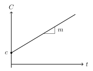
In a linear model $y = mx + c$: the gradient $m$ is the rate of change — how much $y$ increases (or decreases, if $m<0$) each time $x$ increases by $1$. The intercept $c$ is the starting value — the value of $y$ when $x=0$, often a fixed cost, an initial amount, or a starting time. Reading a modelling question is really just identifying which number in the text is the rate and which is the starting value.
Direct proportion: models through the origin
Some quantities aren't just linear — they're directly proportional, written $y \propto x$, meaning $y = kx$ for some constant $k$. This is the special case of a linear model where $c=0$: the line passes exactly through the origin, so $y$ doubles when $x$ doubles, and $y=0$ whenever $x=0$.
A model is one of direct proportion whenever the quantity is genuinely zero when the input is zero — with no fixed starting amount to account for. The circumference of a circle, $C = 2\pi r$, is direct proportion ($k=2\pi$): no radius means no circumference. By contrast, the plumber's call-out fee in the next example is not proportion, because a job of zero hours still costs £40 — the model needs a nonzero intercept.
Building a model from data
Often you're not told $m$ and $c$ directly — you're given two data points (two values of the quantity at two known inputs) and have to find the line through them, exactly as in the previous lesson. The only new step is translating the answer back into the context, and using it to predict values you weren't given.
Using a model to predict a value within the range of the data you were given is called interpolation, and is usually safe. Predicting beyond that range is extrapolation — the model might still be a good fit outside the data, but there's no guarantee, since real quantities often stop increasing at a constant rate eventually. Good modelling answers flag this limitation rather than trusting extrapolated predictions blindly.
Worked example 1
State units for both constants — "£35 per hour" and "£40 fixed fee" — not just the bare numbers. Modelling marks are frequently awarded specifically for interpretation, not just for finding the equation.
Worked example 2
Predicting the height at $t=5$ is interpolation-adjacent (close to the known data), and reasonably safe. But predicting the burn-out time at $t=12$ is a much larger extrapolation — real candles often burn at a slightly different rate as they near the end, so this is a genuine model limitation worth stating in an exam answer.
Worked example 3
Not every worked example needs heavy algebra — sometimes the skill being tested is recognising where a linear model breaks down.
A vague answer like "the model might not be accurate" earns little credit. State which assumption breaks down (constant growth rate) and why it's unreasonable in context (growth naturally slows and stops) — modelling-limitation marks require this level of specificity.
Worked example 4
"Cost the same" means the two linear models intersect — solve them as simultaneous equations, exactly as with any pair of lines.
Plan B has the smaller gradient ($0.5$ vs $2$), so although it starts more expensive (larger intercept), it becomes cheaper for high enough usage. Any two linear models with different gradients cross exactly once — below that crossing point the steeper line is cheaper, above it the shallower line is cheaper. Spotting which side of the break-even point you're on is often the entire point of the question.
Worked example 5
Because a proportional model has only one unknown constant ($k$, since $c=0$ is already fixed), a single data point pins down the whole model — unlike the general linear case, which needs two points to find both $m$ and $c$. Always check first whether a context implies $c=0$; it can save half the work.
Mixing up which variable is the input ($x$) and which is the output ($y$) leads to a model with the gradient and intercept swapped or inverted. Always state clearly what each letter represents before setting up the equation, and check the finished model against the original data as a sanity check.
Check yourself
A tank contains $200$ litres of water and drains at a constant rate. After $8$ minutes it contains $120$ litres. Form a linear model for the volume $V$ litres after $t$ minutes, and use it to predict how long the tank takes to empty completely.
(Hint: the intercept is the starting volume; find the gradient from the one data point given, then solve V = 0.)