Once a hypothesis is set up, the binomial distribution itself decides how surprising a result would have to be before it counts as evidence.
10 min read4 worked examples
Finding a one-tailed critical region
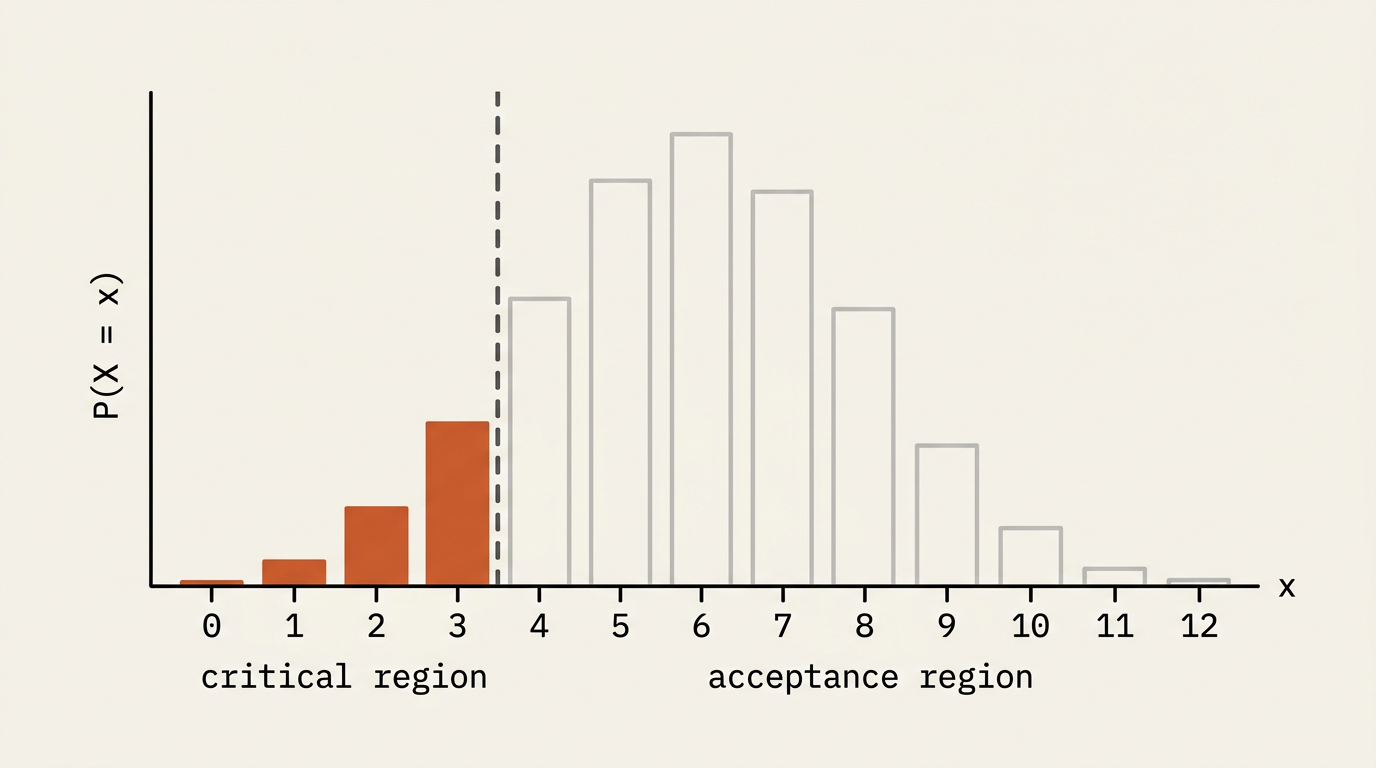
Under $H_0: p=p_0$, the test statistic $X$ follows $B(n,p_0)$. For a test of $H_1: p<p_0$, the critical region is the set of small values of $X$ so unlikely under $H_0$ that observing one would cast doubt on $H_0$. It's built by finding the largest value $c$ such that
$P(X\le c) \le \alpha,$
where $\alpha$ is the significance level. The critical region is then $X \le c$. For a test of $H_1: p>p_0$, the same idea works from the other end: find the smallest $c$ such that $P(X\ge c)\le\alpha$, giving critical region $X\ge c$.
A one-tailed critical region for H₁: p < p₀: the shaded bars at the low end of X are unlikely enough, under H₀, to count as evidence against it.
Why "≤ α", not "= α"
Because $X$ is discrete, it's almost never possible to build a critical region with probability exactly $\alpha$ — the cumulative probabilities jump in discrete steps. The convention is to make the critical region as large as possible without exceeding $\alpha$, which keeps the true chance of wrongly rejecting a correct $H_0$ under control.
Reaching a conclusion
Once the critical region is found, compare the observed value of $X$ against it. If the observed value falls inside the critical region, reject $H_0$ in favour of $H_1$. If not, there is insufficient evidence to reject $H_0$. Either way, state the conclusion back in the context of the original question, not just symbolically.
Strategy — an alternative route using the p-value
Instead of building the whole critical region, you can instead find the probability of a result at least as extreme as the one observed (the p-value), and compare it directly to $\alpha$. Both approaches always agree — the critical-region method and the p-value method are two ways of asking the same question.
Worked example 1
Finding a critical region
A machine is claimed to produce 30% defective items. To test $H_0: p=0.3$ against $H_1: p<0.3$ at the 5% significance level, a sample of $n=20$ items is checked. Find the critical region.
MethodFind the largest c with P(X≤c) ≤ 0.05, under X~B(20,0.3)
1
Under $H_0$: $X\sim B(20,0.3)$.
The claimed value under the null hypothesis.
2
Using cumulative binomial probabilities: $P(X\le2) \approx 0.0355$, $P(X\le3)\approx0.1071$.
Read from tables or a calculator's binomial cdf.
3
$P(X\le2)\approx0.0355 \le 0.05$, but $P(X\le3)\approx0.1071 > 0.05$.
Test successive values of c against α.
4
So the critical region is $X\le2$.
The largest c that still satisfies the ≤ α condition.
▪ found
Examiner's eye
Always show both the boundary value's probability and the next value's probability — this proves the critical region is the largest possible one satisfying $P(X\le c)\le\alpha$, which is exactly what the mark scheme is checking for.
Worked example 2
Completing the test
Using the critical region $X\le2$ found above, a sample of 20 items is checked and $1$ is found defective. Complete the hypothesis test and state a conclusion in context.
MethodCompare the observed value against the critical region
1
Observed value: $X=1$.
The actual sample result.
2
The critical region is $X\le2$, and $1\le2$, so the observed value lies in the critical region.
Compare against the region found previously.
3
There is sufficient evidence to reject $H_0$ in favour of $H_1$ — the data suggests the true proportion of defective items is lower than the claimed 30%.
Conclusion stated in the context of the original claim.
▪ concluded
The key insight
The conclusion must be written in words about the original scenario ("the proportion of defective items is lower than claimed"), not left as "reject $H_0$" — a symbolic-only conclusion, however correct the working, typically loses the final mark of a hypothesis-testing question.
Worked example 3
An upper-tail critical region
A vaccine is claimed to be effective in 70% of cases. A researcher tests $H_0: p=0.7$ against $H_1: p>0.7$ at the 10% level, with $n=15$. Given $P(X\ge13)\approx0.1268$ and $P(X\ge12)\approx0.2969$, find the critical region.
MethodFind the smallest c with P(X≥c) ≤ 0.10
1
For an upper-tail test, we need the smallest $c$ with $P(X\ge c)\le0.10$.
The mirror-image rule to the lower-tail case.
2
$P(X\ge13)\approx0.1268 > 0.10$, so $c=13$ doesn't satisfy the condition.
Test the given values in order.
3
Since $P(X\ge12)\approx0.2969$ is even larger, we instead need to check $P(X\ge14)$, which must be smaller still than $P(X\ge13)$.
Move to the next candidate upward, since 13 failed.
4
Since $P(X\ge13)\approx0.1268$ already exceeds $0.10$, the critical region starts at the next value up: $X\ge14$.
13 is too likely; 14 is the smallest value satisfying the condition.
▪ found
Common mistake
For an upper-tail test ($H_1: p>p_0$), the inequality direction flips compared to the lower-tail case — you're finding the smallest $c$ with $P(X\ge c)\le\alpha$, not the largest. Mixing up the two directions is one of the most common errors in this topic.
Worked example 4
Using the p-value method · Challenge
A coin is tested for bias toward tails: $H_0: p=0.5$, $H_1: p<0.5$ (where $p$ is the probability of heads), at the 5% level, with $n=18$ tosses. The coin shows $5$ heads. Given $P(X\le5) \approx 0.0481$ where $X\sim B(18,0.5)$, use the p-value method to reach a conclusion.
MethodCompare the p-value directly to the significance level
1
The p-value is the probability of a result at least as extreme as observed: $P(X\le5) \approx 0.0481$.
"At least as extreme" for a lower-tail test means X ≤ 5.
2
Compare to the significance level: $0.0481 < 0.05$.
p-value below α.
3
Since the p-value is less than $5\%$, there is sufficient evidence to reject $H_0$ — the coin appears biased toward tails.
Small p-value means the observed result is unusual under H₀.
▪ concluded
Look deeper — the p-value method and critical region method always agree
Since $P(X\le5)\approx0.0481\le0.05$, the critical region built from this significance level would necessarily include $X=5$ too — both methods are really the same test, viewed from two different angles. The p-value method is often faster when only one specific observed value needs testing, rather than the full critical region.
Common mistake
The critical region is built from $H_0$'s distribution, $B(n,p_0)$ — never from any estimate based on the sample itself. And "$X\le2$" as a final answer, without first stating the distribution it was derived from, is an incomplete critical region — always show the distribution and the working, not just the final inequality.
Check yourself
To test $H_0: p=0.4$ against $H_1: p<0.4$ at the 5% level with $n=25$, given $P(X\le5)\approx0.0294$ and $P(X\le6)\approx0.0736$ for $X\sim B(25,0.4)$, find the critical region. (Hint: find the largest c with P(X≤c) ≤ 0.05.)