Critical Values
A hypothesis test needs a hard boundary — a line drawn through the distribution that separates "unremarkable" from "so unlikely it counts as evidence". That line is the critical value.
Critical region and acceptance region
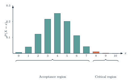
Under $H_0$, the test statistic $X$ follows a known distribution — here, always binomial. The critical region is the set of values of $X$ so extreme that, if observed, they would cause $H_0$ to be rejected. Everything outside it is the acceptance region: values consistent enough with $H_0$ that there's no reason to doubt it.
Critical value and actual significance level
The critical value is the first value of $X$ that falls inside the critical region — the boundary itself. In the diagram above, the critical value is $8$.
Because $X$ is discrete, the critical region's total probability almost never lands exactly on the stated significance level $\alpha$ — it's built to be as close as possible to $\alpha$ without exceeding it. The actual probability of the test statistic falling in the critical region, assuming $H_0$ is true, is called the actual significance level of the test, and it's usually slightly below the stated level.
The stated significance level (5%, say) is a target, not a guarantee — quoting the actual significance level shows you understand that a discrete test can only approximate it, and lets you judge exactly how cautious (or how permissive) a particular test really is.
Finding a critical region
To find the critical region for $H_1:p>p_0$ at significance level $\alpha$: find the smallest value $c$ such that $P(X\ge c)\le\alpha$. Everything from $c$ upward is the critical region. For $H_1:p<p_0$, the logic mirrors this from the other end: find the largest value $c$ such that $P(X\le c)\le\alpha$.
Worked example 1
Always show the probability just outside the critical region too (here, $P(X\ge5)=0.0580$) — this proves the region you've chosen is the largest possible one still under 5%, which is exactly what a mark scheme checks for.
Worked example 2
The method is a mirror image of the upper-tail case: instead of building the region up from the largest values of $X$, it's built up from the smallest. Deciding which end to search from comes entirely from the direction stated in $H_1$.
Do not stop at the first value where the cumulative probability looks "close to" $\alpha$ — always check the boundary value and its neighbour to confirm the region is as large as possible without exceeding $\alpha$. A critical region built from a value with $P>\alpha$ is simply wrong, however close it looks.
Check yourself
$X\sim B(12, 0.25)$ is used to test $H_0:p=0.25$ against $H_1:p<0.25$ at the 5% significance level. Given $P(X\le0)=0.0317$ and $P(X\le1)=0.1584$, find the critical region and the actual significance level.
(Hint: find the largest c with P(X≤c) ≤ 0.05.)