Linearising with Logs
Taking logs turns power laws and exponential laws into straight lines — so the hidden constants read straight off a gradient and intercept.
Turning curves into straight lines
Straight lines are easy: plot the data, read the gradient and intercept, done. Curves are not. But two very common non-linear relationships — $y = ax^n$ (a power law) and $y = kb^x$ (an exponential law) — can be turned into straight lines by taking logs. Once linear, you plot the transformed data, fit a line, and read the unknown constants off its gradient and intercept. This is how scientists find the hidden law behind a set of measurements.
The laws of logs split products and pull powers down to the front. Applied to $y = ax^n$ or $y = kb^x$, they separate the variable term from the constants and drop any exponent into a multiplier — exactly the structure of $Y = mX + c$. The curve doesn't change; you're just plotting $\log y$ (and sometimes $\log x$) instead of the raw values, and in those new coordinates the same relationship looks straight.
Case 1 — the power law y = axⁿ
Take logs of both sides and apply the product and power laws:
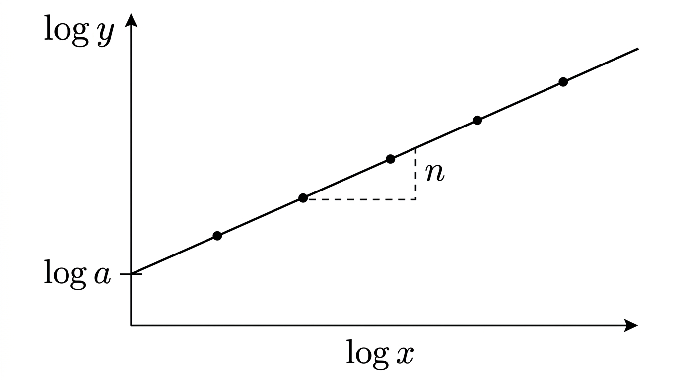
Compare with $Y = mX + c$: plotting $\log y$ against $\log x$ gives a straight line with gradient $n$ and vertical intercept $\log a$. So the power $n$ is the gradient, and $a = 10^{\text{intercept}}$.
Case 2 — the exponential law y = kbˣ
Here the variable is already in the exponent, so take logs and use the power law on $b^x$:
This time plot $\log y$ against $x$ (not $\log x$) — the line has gradient $\log b$ and intercept $\log k$. So $b = 10^{\text{gradient}}$ and $k = 10^{\text{intercept}}$.
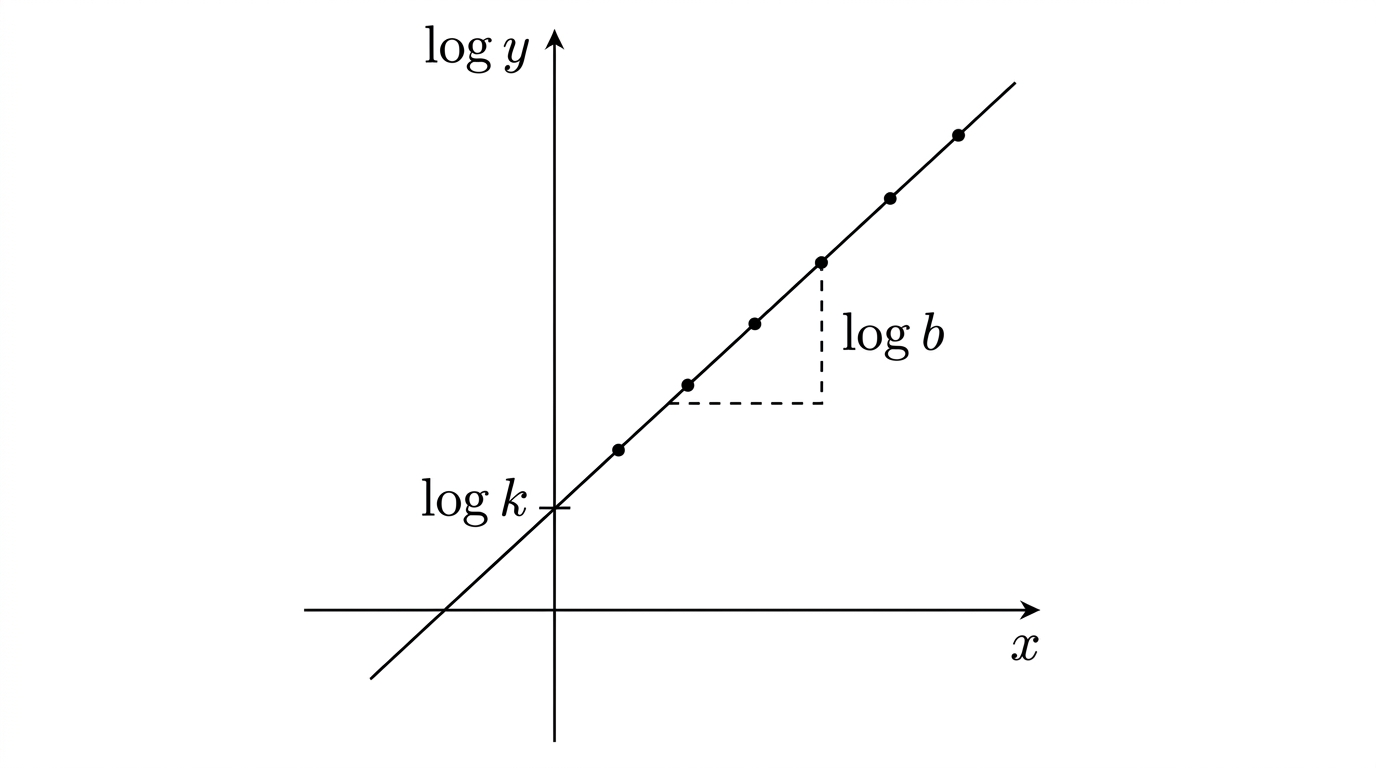
The single decision is what to plot. If the model is a power of $x$ ($y=ax^n$), take logs of both variables: $\log y$ against $\log x$. If the variable is in the exponent ($y=kb^x$), take the log of $y$ only: $\log y$ against $x$. A quick test: is $x$ raised to a fixed power, or is a fixed number raised to the power $x$? The first is log–log; the second is log–linear.
Worked example 1
The gradient gives the power directly — no undoing needed — but the intercept gives $\log a$, so you must raise $10$ to it to recover $a$. Mixing these up (reading $a$ as the intercept, or trying to "un-log" the gradient) is the classic error. Gradient → power, intercept → $10^{\text{intercept}}$ for the coefficient.
Worked example 2
Contrast this with example 1. There, the power law needed $\log y$ against $\log x$ and the gradient was the power. Here, the exponential law needs $\log y$ against $x$, and now both gradient and intercept must be un-logged, because $b$ and $k$ each sit inside a log. The structure of the model — power of $x$ versus number to the power $x$ — decides both the axes and what you do with the results.
Worked example 3
Every technique here is the equation of a straight line lesson applied to $\log$-transformed coordinates: gradient from two points, intercept by substituting one back in. The only extra step is un-logging at the end to recover the real-world constants. If you can find the equation of a line through two points, you can fit any power or exponential law to data.
Choosing the wrong axes is the big one: $y=ax^n$ needs $\log y$ vs $\log x$ (log–log), while $y=kb^x$ needs $\log y$ vs $x$ (log–linear). Plotting $\log x$ when you should plot $x$ turns a straight line into a curve. The second trap is forgetting to un-log the intercept — the intercept is $\log a$ or $\log k$, so the constant is $10$ to that power, not the intercept value itself.
Check yourself
Data believed to follow $y = ax^{n}$ is plotted as $\log y$ against $\log x$, giving a straight line of gradient $2$ passing through $(1,\ 2.3)$. Find $a$ and $n$.
(Hint: gradient is $n$; find the intercept $\log a$ using the point, then un-log.)
The gradient $2$ gave the power immediately. The intercept had to be computed from the point (it's $\log a = 0.3$), then un-logged to $a = 10^{0.3} \approx 2$.