Exponential Growth & Decay
When something changes at a rate proportional to its size, an exponential models it. Find the constants from data, then predict — and know the model's limits.
Modelling change that's proportional to size
Many real quantities grow or shrink at a rate proportional to how much is currently there: a population with more individuals breeds faster; a radioactive sample with more atoms decays faster; savings earning continuous interest grow faster the larger the balance. All of these are described by an exponential model
where $t$ is time, $A$ is the initial amount (the value when $t=0$), and $k$ is a constant setting the pace. If $k>0$ the quantity grows; if $k<0$ it decays. The whole topic is reading this model, finding its constants from data, and interpreting what it predicts.
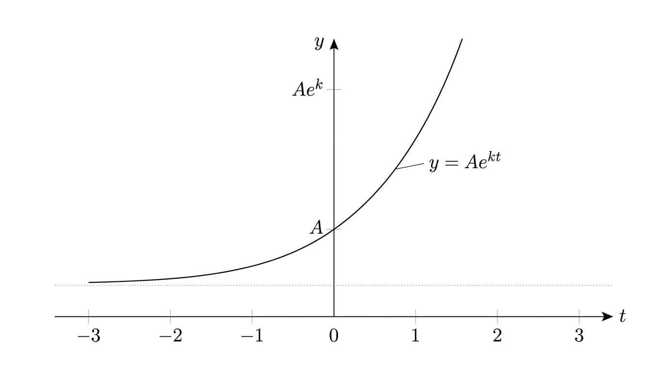
Setting $t = 0$ in $y = Ae^{kt}$ gives $y = Ae^{0} = A$, since $e^0 = 1$. So $A$ is always the amount you start with — the population at the first census, the mass before decay begins, the opening balance. Whenever a question says "initially" or "at the start", it's telling you the value of $y$ when $t=0$, which pins down $A$ immediately.
The shape of the two behaviours
Almost every modelling question gives you two pieces of information. Use the "initial" value to read off $A$ straight away. Then substitute the second data point and solve for $k$ using natural logs — since the unknown $k$ sits in the exponent, taking $\ln$ of both sides is what frees it. With $A$ and $k$ known, the model is complete and you can answer anything else it asks.
Worked example 1
Round sensibly and in context: $5510$ bacteria (a count, so a whole number), and $7.49$ hours if asked to 3 s.f. Watch that the $0.4$ multiplies $t$ inside the exponent — after taking logs you get $0.4t$, and must divide by $0.4$ at the end. Forgetting that division is the most frequent error here.
Worked example 2
The value of $k$ came out negative, which is the signature of decay — as expected, since the mass is falling. That negative sign isn't optional: if you'd got a positive $k$ here, you'd know something went wrong. The two data points did their jobs cleanly — the "initial" one fixed $m_0$, the later one fixed $k$ — which is the standard two-step every modelling question follows.
Worked example 3
Unbounded exponential growth is only realistic over a limited window. The exam explicitly rewards criticising models: noting that a real population can't grow forever, that a decaying quantity approaches but never truly hits zero, or that a predicted value falls outside a sensible range. A good answer states what the model does well and where it breaks down — not just a number.
When solving for a constant in the exponent, don't forget to divide by its coefficient after taking logs: from $e^{10k} = 0.75$ you get $10k = \ln 0.75$, so $k = \tfrac{1}{10}\ln 0.75$ — not $k = \ln 0.75$. And read $A$ as the value at $t=0$, not the value in the first year mentioned: "initially $80$ g" means $t=0$, so $m_0 = 80$ directly, with no calculation needed.
Check yourself
The value $£V$ of a car after $t$ years is modelled by $V = 18\,000 e^{kt}$. After $3$ years the car is worth $£12\,000$. Find $k$, and use it to estimate the car's value after $8$ years.
(Hint: substitute the 3-year data to find $k$, then substitute $t=8$.)
The negative $k$ signals depreciation, as expected for a car losing value. Substituting $t=8$ into the completed model gives roughly $£6100$ — a realistic figure over the short-to-medium term.