Statistics · Statistical Distributions · Year 1

The Binomial Distribution

Counting successes across a fixed number of identical, independent trials happens so often it earns its own named distribution — and its own one-line formula.

11 min read 4 worked examples

The binomial conditions

A random variable follows a binomial distribution, written $X \sim B(n,p)$, when four conditions all hold:

A fixed number of trials, $n$.
Each trial has only two outcomes — "success" and "failure".
A constant probability of success, $p$, on every trial.
The trials are independent of each other.

$X$ then counts the number of successes across the $n$ trials.

Checking the conditions is not optional

Before using the binomial formula, exam questions frequently require you to justify that a scenario is binomial — and to flag when it isn't. Sampling without replacement from a small population, for instance, breaks the "constant $p$" and "independent" conditions simultaneously, since removing an item changes the proportions left for the next draw.

The binomial probability formula

For $X \sim B(n,p)$, the probability of exactly $r$ successes is

$P(X=r) = \binom{n}{r} p^r (1-p)^{n-r}, \qquad r=0,1,2,\ldots,n.$

Each part has a role: $\binom{n}{r}$ counts how many ways $r$ successes can be arranged among $n$ trials; $p^r$ is the probability of those $r$ successes all happening; $(1-p)^{n-r}$ is the probability of the remaining $n-r$ trials all being failures.
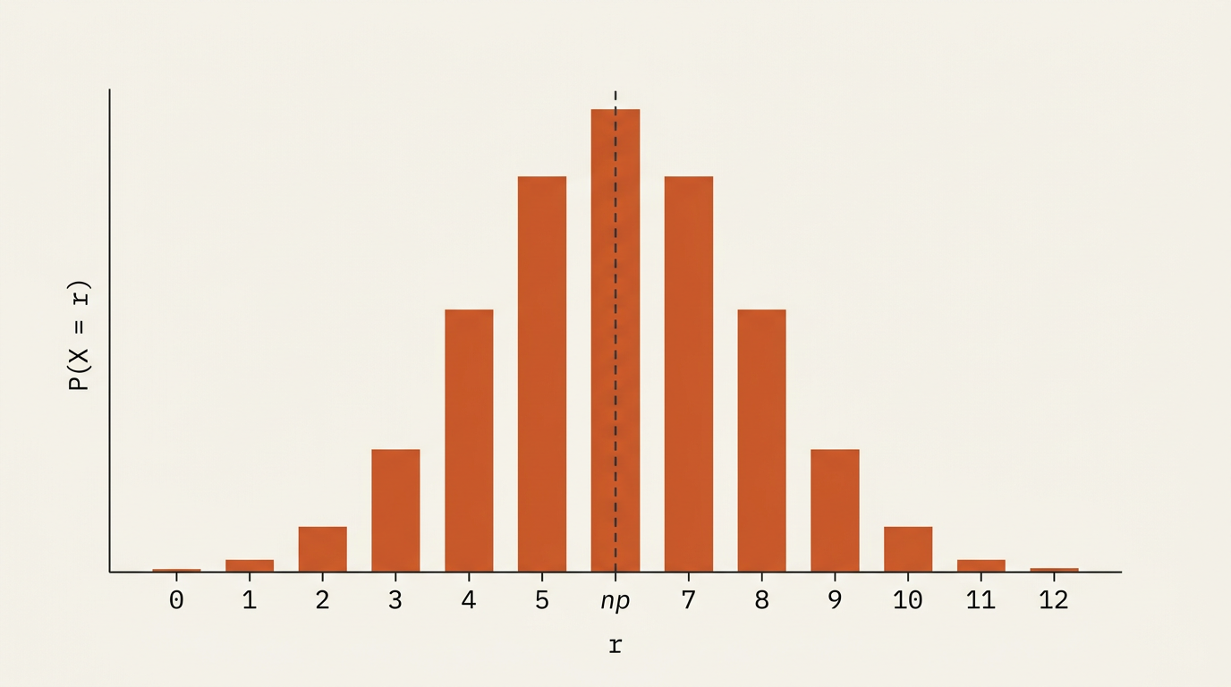
A bar chart showing a binomial probability distribution, with bars at integer values on the horizontal axis rising to a peak near the mean and falling away symmetrically on either side, representing P(X=r) against r.
The probability distribution of a binomial random variable B(n, p): a bar at each integer value of r, peaking around the mean np.

Mean and using tables or a calculator

For $X\sim B(n,p)$, the mean is simply $E(X) = np$ — the number of trials times the probability of success, matching intuition directly. Cumulative probabilities such as $P(X\le r)$ are usually found from a calculator's binomial cumulative distribution function, or from statistical tables, rather than by adding individual terms by hand.

Strategy — translate "at least", "at most", "more than" carefully

$P(X\ge r)$, $P(X\le r)$, $P(X>r)$ and $P(X<r)$ are all subtly different, and each needs converting to a form a cumulative table or calculator function actually computes. A reliable approach: rewrite everything in terms of $P(X\le k)$ for some $k$, using $P(X\ge r)=1-P(X\le r-1)$ and $P(X>r)=1-P(X\le r)$.

Worked example 1

An individual binomial probability
A fair coin is tossed $8$ times. Find the probability of getting exactly $5$ heads.
MethodIdentify n, p, r, then substitute into the formula
1
$X\sim B(8, 0.5)$: $n=8$ tosses, $p=0.5$ per toss, independent, two outcomes.
Confirms all four binomial conditions.
2
$P(X=5) = \dbinom{8}{5}(0.5)^5(0.5)^{3}$.
r=5 successes, n−r=3 failures.
3
$\dbinom{8}{5}=56$, so $P(X=5) = 56\times(0.5)^8 = \dfrac{56}{256} = 0.21875$.
Combine the coefficient with (0.5)^8.
▪ solved
Examiner's eye

State the distribution ($X\sim B(8,0.5)$) explicitly before calculating — this is often a method mark on its own, and forces you to double-check $n$, $p$, and what counts as "success" before the arithmetic begins.

Worked example 2

A cumulative probability
A factory finds that 10% of items it produces are faulty. In a random sample of 15 items, let $X$ be the number of faulty items. Find $P(X\le 2)$.
MethodSum the individual probabilities for X = 0, 1, 2
1
$X\sim B(15, 0.1)$.
15 independent items, constant 10% fault rate.
2
$P(X=0) = (0.9)^{15} \approx 0.2059$.
No successes: (1−p) to the power n.
3
$P(X=1) = \dbinom{15}{1}(0.1)^1(0.9)^{14} \approx 15\times0.1\times0.2288 \approx 0.3432$.
Exactly one faulty item.
4
$P(X=2) = \dbinom{15}{2}(0.1)^2(0.9)^{13} \approx 105\times0.01\times0.2542 \approx 0.2669$.
Exactly two faulty items.
5
$P(X\le2) = 0.2059+0.3432+0.2669 \approx 0.816$.
Sum the three probabilities.
▪ solved
The key insight

In practice, a calculator's binomial cumulative distribution function returns $P(X\le 2)$ directly from $n$, $p$ and $2$ in a single step — the term-by-term addition here shows what that function is doing internally, but exam technique should default to the calculator function once the distribution is correctly identified.

Worked example 3

Checking the binomial conditions
A bag contains 5 red and 3 blue counters. Three counters are drawn without replacement. Explain why the number of red counters drawn does not follow a binomial distribution.
MethodCheck each condition against the sampling method
1
Without replacement, the probability of drawing red changes after each draw, since the bag's contents change.
Directly contradicts "constant p".
2
This also means each draw's outcome affects the probabilities for the next draw — the draws are not independent.
Contradicts the independence condition too.
3
Two of the four binomial conditions fail, so this situation cannot be modelled as binomial.
Both failures stem from the same root cause: no replacement.
▪ explained
Common mistake

"Without replacement" is the single most common way a scenario fails to be binomial — always check for it explicitly. (This kind of situation instead follows a different model, the hypergeometric distribution, which sits beyond this course.)

Worked example 4

Finding an unknown parameter · Challenge
$X\sim B(n, 0.3)$, and $E(X)=9$. Find $n$, then find $P(X=3)$.
MethodUse E(X)=np to find n, then apply the formula
1
$E(X) = np \Rightarrow 9 = n(0.3) \Rightarrow n=30$.
Rearrange the mean formula.
2
$X\sim B(30, 0.3)$. $P(X=3) = \dbinom{30}{3}(0.3)^3(0.7)^{27}$.
Substitute n=30, r=3.
3
$\dbinom{30}{3}=4060$, and $(0.3)^3(0.7)^{27} \approx 0.027\times0.000420 \approx 0.0000113$.
Evaluate each piece.
4
$P(X=3) \approx 4060\times0.0000113 \approx 0.0459$.
Multiply the coefficient by the probability piece.
▪ solved
Look deeper — why P(X=3) is small despite a plausible-sounding value

With $n=30$ and $p=0.3$, the mean number of successes is $9$ — so $X=3$ is far below the "typical" outcome, and its probability is correspondingly small. Values of $X$ close to $np$ carry the most probability; values far from it, in either direction, are increasingly unlikely, which is exactly the shape shown in the bar chart earlier in this lesson.

Common mistake

$\binom{n}{r}$ counts arrangements, not probability — never forget it, or the formula collapses into "probability of one specific sequence of successes and failures" rather than "probability of $r$ successes in any order". And always double check whether a question wants $P(X=r)$ (exact) or a cumulative probability — these need entirely different calculator functions.

Check yourself

$X\sim B(10, 0.4)$. Find $P(X=4)$ and $E(X)$.
(Hint: use the binomial formula for P(X=4), and E(X)=np for the mean.)

Method
1
$P(X=4) = \dbinom{10}{4}(0.4)^4(0.6)^6 = 210\times0.0256\times0.046656 \approx 0.2508$.
2
$E(X) = np = 10\times0.4=4$.
Mean of a binomial distribution.
▪ solved